Use simple linear regression to describe the relationship between a quantitative predictor and quantitative response variable.
Estimate the slope and intercept of the regression line using the least squares method.
Interpret the slope and intercept of the regression line.
Use R to fit and summarize regression models.
Computation set up
# load packageslibrary(tidyverse) # for data wranglinglibrary(ggformula) # for plottinglibrary(broom) # for formatting model outputlibrary(knitr) # for formatting tables# set default theme and larger font size for ggplot2ggplot2::theme_set(ggplot2::theme_bw(base_size =16))# set default figure parameters for knitrknitr::opts_chunk$set(fig.width =8,fig.asp =0.618,fig.retina =3,dpi =300,out.width ="80%")
Data
DC Bikeshare
Our data set contains daily rentals from the Capital Bikeshare in Washington, DC in 2011 and 2012. It was obtained from the dcbikeshare data set in the dsbox R package.
We will focus on the following variables in the analysis:
Click here for the full list of variables and definitions.
Let’s complete Exercises 2-6 together
Data prep
Exercise 2: Recode season as a factor with names instead of numbers (livecode)
Remember:
Think of |> as “and then”
mutate creates new columns and changes (mutates) existing columns
R calls categorical data “factors”
bikeshare <-read_csv("../data/dcbikeshare.csv") |>mutate(season =case_when( season ==1~"winter", season ==2~"spring", season ==3~"summer", season ==4~"fall" ),season =factor(season))
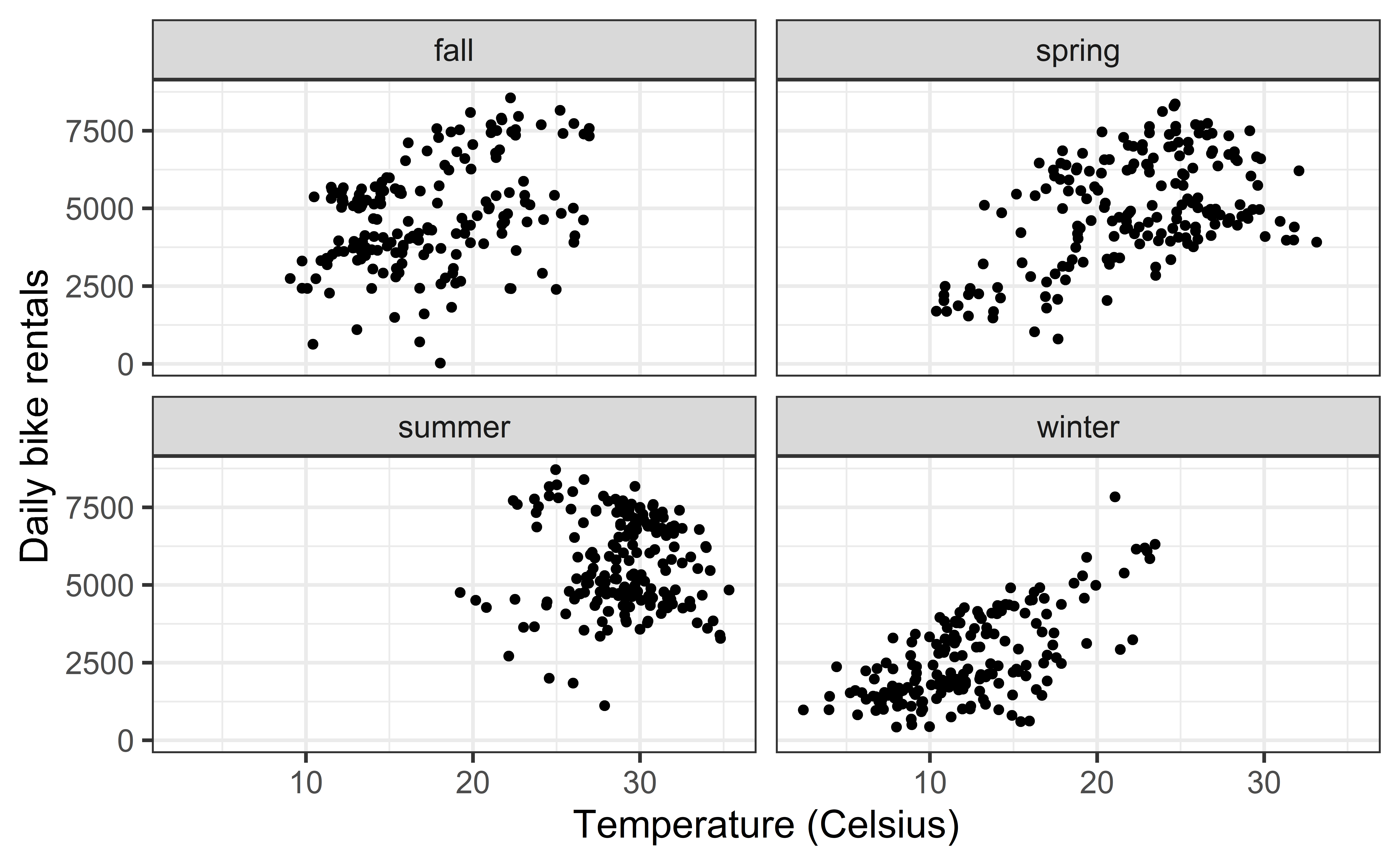
Exploratory data analysis (Exercise 3)
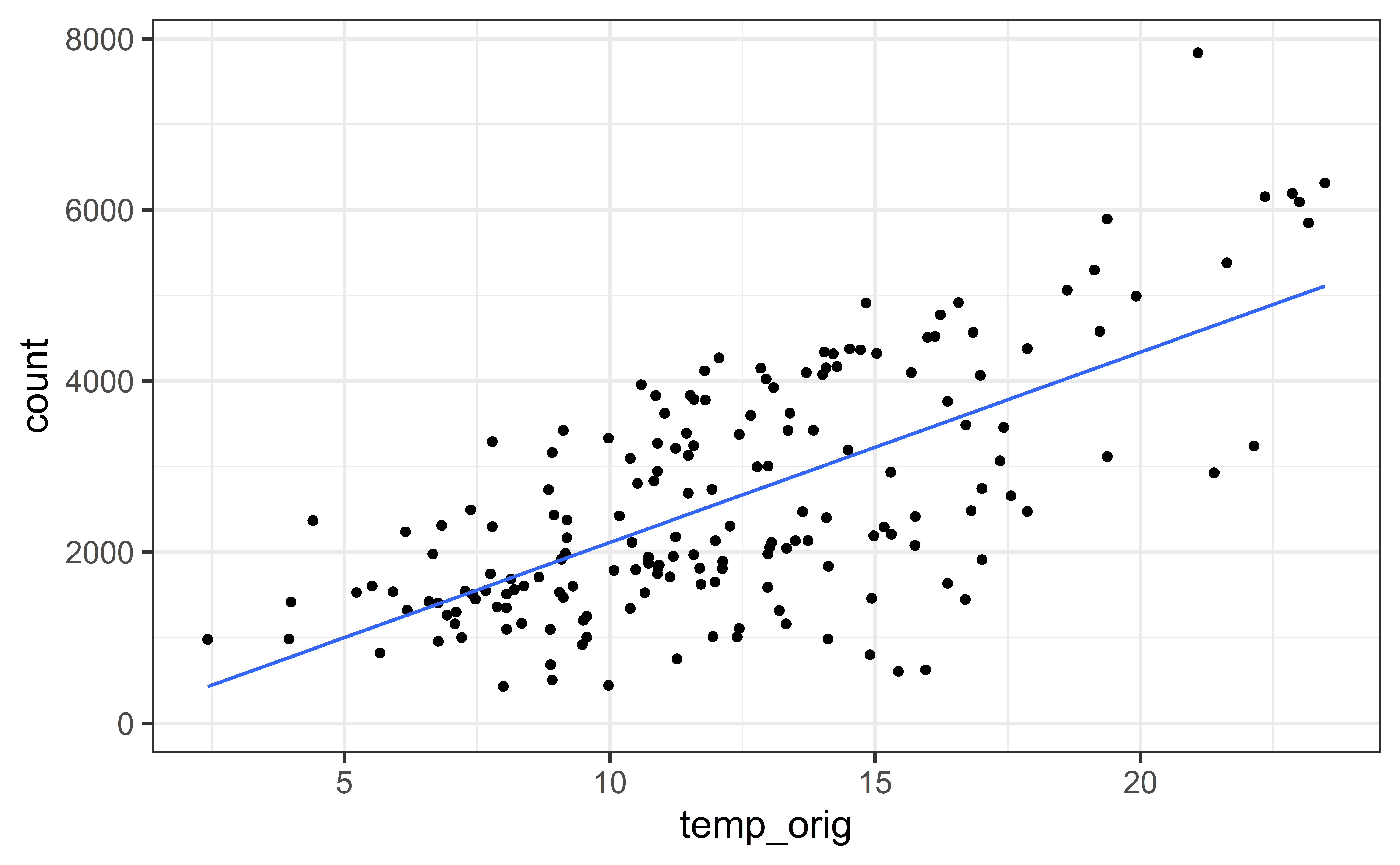
gf_point(count ~ temp_orig | season, data = bikeshare) |>gf_labs(x ="Temperature (Celsius)",y ="Daily bike rentals")
Exploratory data analysis (Exercise 3)
gf_point(count ~ temp_orig | season, data = bikeshare) |>gf_labs(x ="Temperature (Celsius)",y ="Daily bike rentals")
More data prep
(Exercise 5) Filter your data for the season with the strongest relationship and give the resulting data set a new name
winter <- bikeshare |>filter(season =="winter")
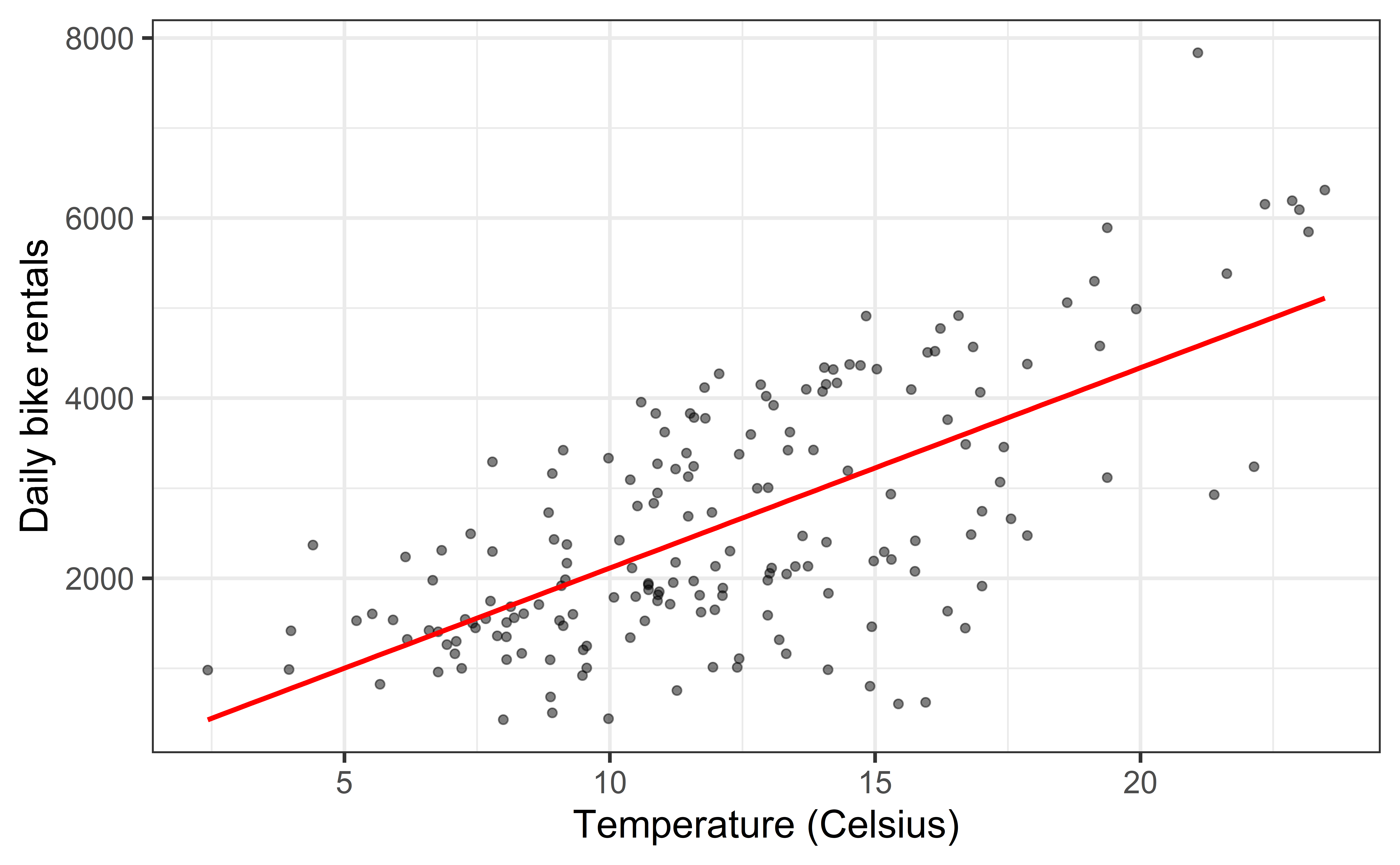
Rentals vs Temperature
Goal: Fit a line to describe the relationship between the temperature and the number of rentals in winter.
Why fit a line?
We fit a line to accomplish one or both of the following:
Prediction
How many rentals are expected when it’s 10 degrees out?
Inference
Is temperature a useful predictor of the number of rentals? By how much is the number of rentals expected to change for each degree Celsius?
Population vs. Sample
Population: The set of items or events that you’re interested in and hoping (able) to generalize the results of your analysis to.
Sample: The set of items that you have data for.
Representative Sample: A sample that looks like a small version of your population.
Goal: Build a model from your sample which generalizes to your population.
Terminology
Response, Y: variable describing the outcome of interest
Predictor, X: variable we use to help understand the variability in the response
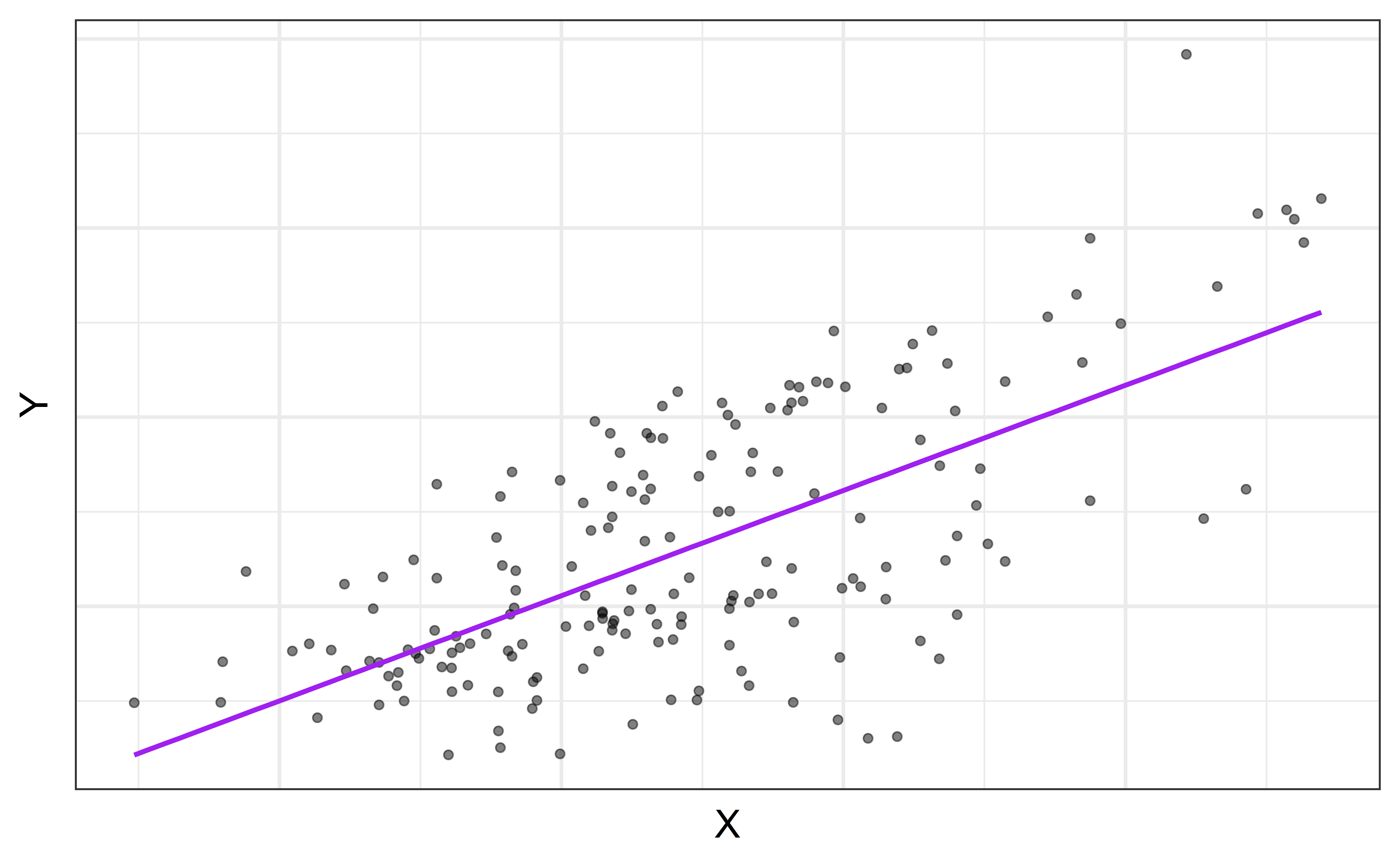
Regression model
Regression model: a function that describes the relationship between a quantitative response, \(Y\), and the predictor, \(X\) (or many predictors).
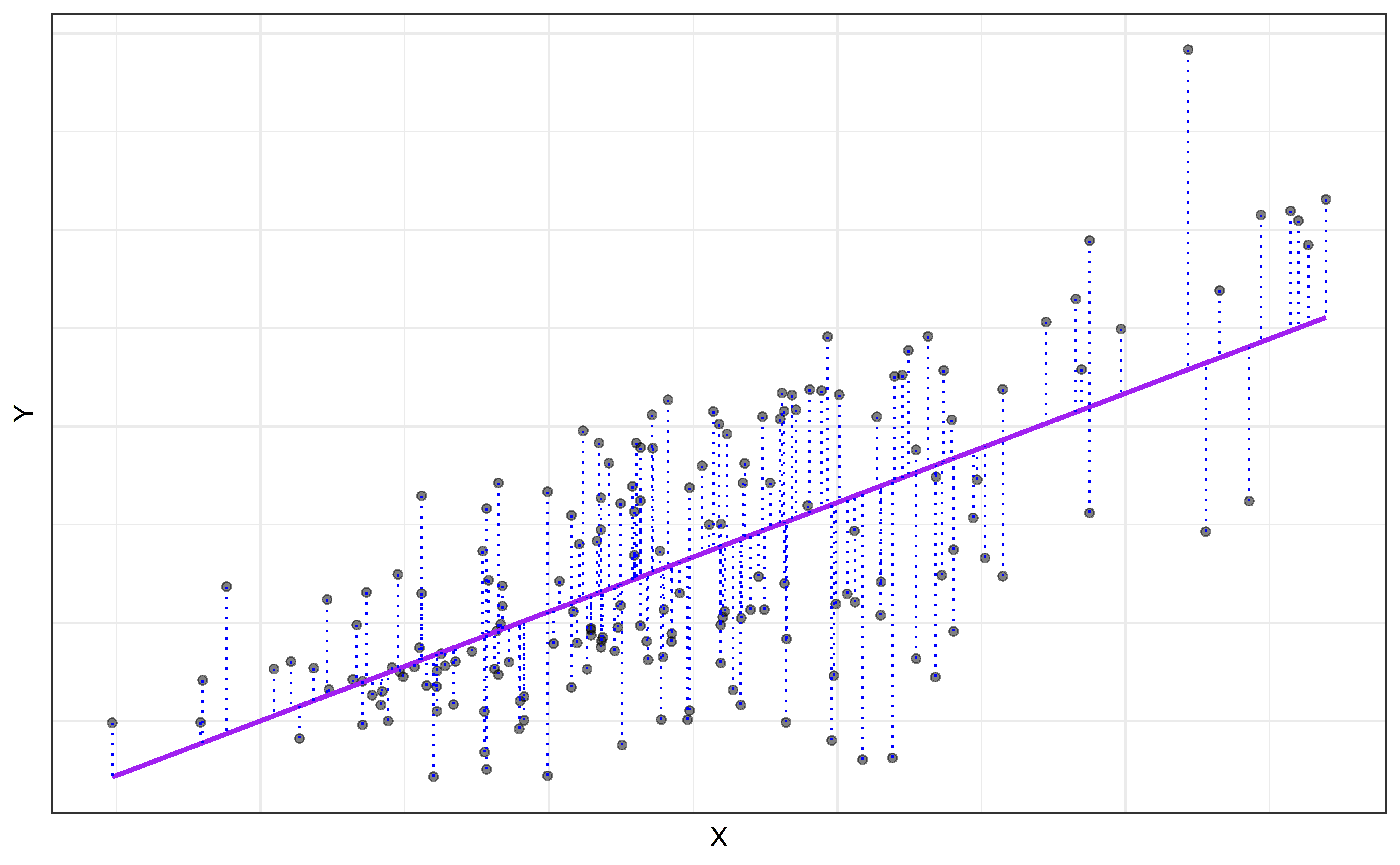
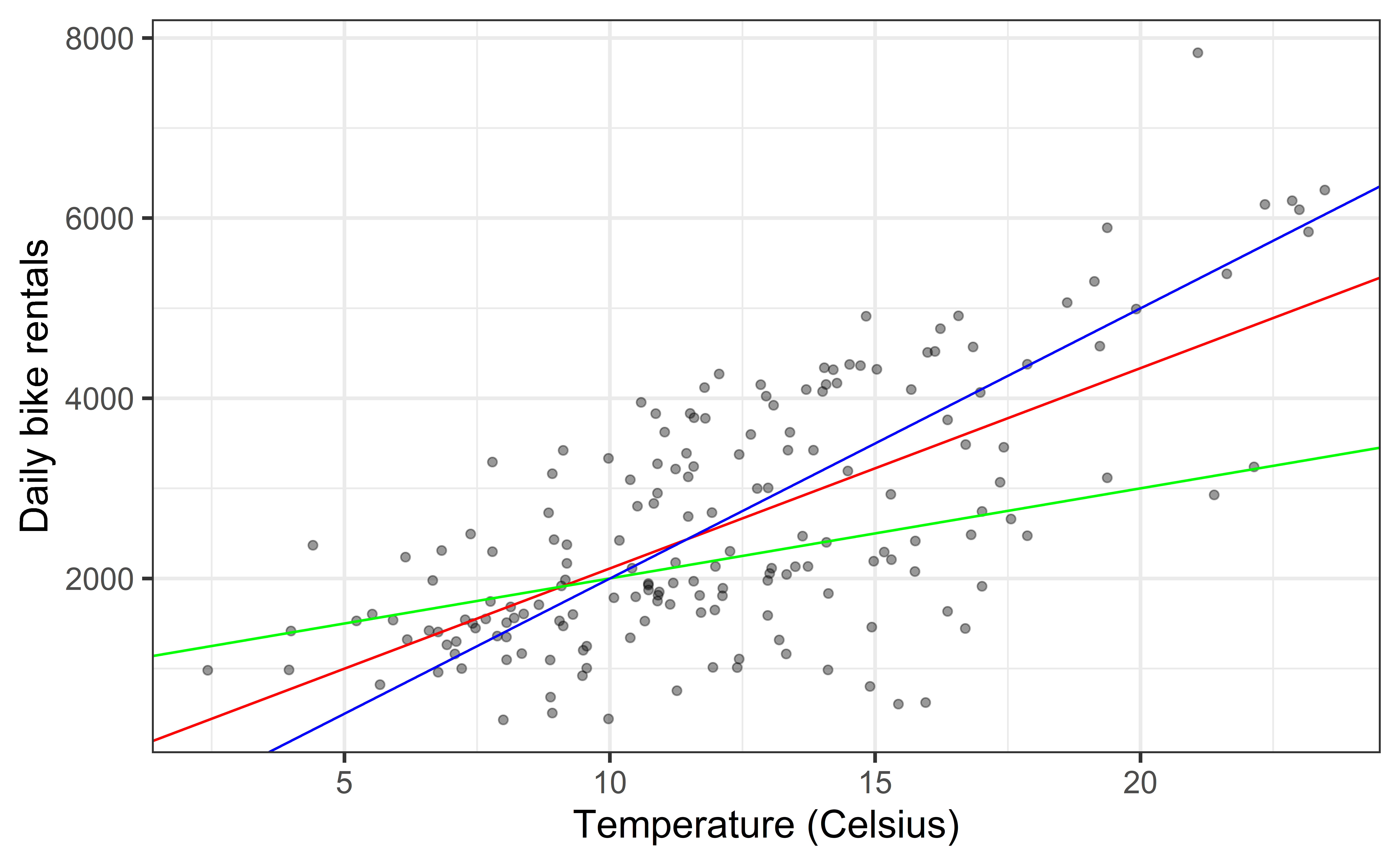
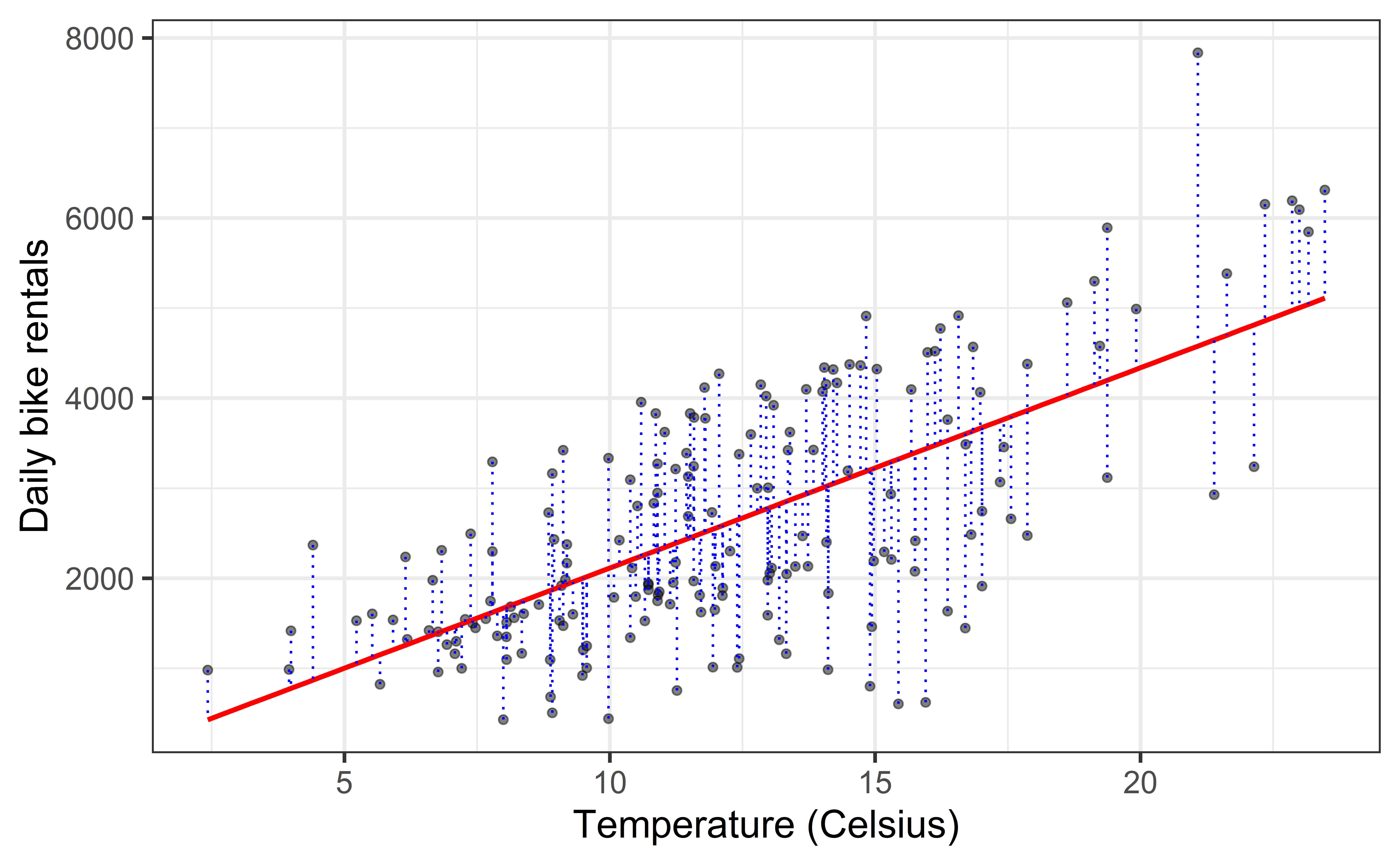
Least squares line is the one that minimizes the sum of squared residuals
Slope and intercept
Properties of least squares regression
Passes through center of mass point, the coordinates corresponding to average \(X\) and average \(Y\): \(\hat{\beta}_0 = \bar{Y} - \hat{\beta}_1\bar{X}\)
Slope has same sign as the correlation coefficient: \(\hat{\beta}_1 = r \frac{s_Y}{s_X}\)
\(r\): correlation coefficient
\(s_Y, s_X\): sample standard deviations of \(X\) and \(Y\)
Sum of the residuals is zero: \(\sum_{i = 1}^n e_i \approx 0\)