Multiple Logistic Regression

Prof. Eric Friedlander

Topics

Extending what we’ve learned to logistic regression models with multiple predictors

Complete all of AE 12 using slides as needed.

Computational setup

# load packages
library(tidyverse)
library(broom)
library(openintro)
library(knitr)
library(kableExtra)  # for table embellishments
library(Stat2Data)   # for empirical logit

# set default theme and larger font size for ggplot2
ggplot2::theme_set(ggplot2::theme_bw(base_size = 20))

Data

Risk of coronary heart disease

This data set is from an ongoing cardiovascular study on residents of the town of Framingham, Massachusetts. We want to examine the relationship between various health characteristics and the risk of having heart disease.

TenYearCHD:
- 1: Developed heart disease in next 10 years
- 0: Did not develop heart disease in next 10 years
age: Age at exam time (in years)
education: 1 = Some High School, 2 = High School or GED, 3 = Some College or Vocational School, 4 = College

Data prep

heart_disease <- read_csv("../data/framingham.csv") |>
  select(TenYearCHD, age, education) |>
  drop_na() |> 
  mutate(education = as.factor(education))

heart_disease |> head() |> kable()

TenYearCHD	age	education
0	39	4
0	46	2
0	48	1
1	61	3
0	46	3
0	43	2

Coefficient Interpretation

Model output

risk_fit <- glm(TenYearCHD ~ age + education, 
      data = heart_disease, family = "binomial")

risk_fit |> tidy() |> kable(digits = 3)

term	estimate	std.error	statistic	p.value
(Intercept)	-5.385	0.308	-17.507	0.000
age	0.073	0.005	13.385	0.000
education2	-0.242	0.112	-2.162	0.031
education3	-0.235	0.134	-1.761	0.078
education4	-0.020	0.148	-0.136	0.892

\[ \small{\log\Big(\frac{\hat{\pi}}{1-\hat{\pi}}\Big) = -5.385 + 0.073 ~ \text{age} - 0.242 ~ \text{ed2} - 0.235 ~ \text{ed3} - 0.020 ~ \text{ed4}} \]

Model Interpretation

risk_fit <- glm(TenYearCHD ~ age + education, 
      data = heart_disease, family = "binomial")

risk_fit |> tidy() |> kable(digits = 3)

term	estimate	std.error	statistic	p.value
(Intercept)	-5.385	0.308	-17.507	0.000
age	0.073	0.005	13.385	0.000
education2	-0.242	0.112	-2.162	0.031
education3	-0.235	0.134	-1.761	0.078
education4	-0.020	0.148	-0.136	0.892

As age increases by a year, the typical log-odds of developing coronary heart disease within the next 10 years increases by 0.073 for patients with the same level of education.

As age increases by a year, the typical odds of developing coronary heart disease within the next 10 years increases by a factor of \(\exp(0.073)\approx 1.08\) (i.e. 8%) for patients with the same level of education.

Model Interpretation

risk_fit <- glm(TenYearCHD ~ age + education, 
      data = heart_disease, family = "binomial")

risk_fit |> tidy() |> kable(digits = 3)

term	estimate	std.error	statistic	p.value
(Intercept)	-5.385	0.308	-17.507	0.000
age	0.073	0.005	13.385	0.000
education2	-0.242	0.112	-2.162	0.031
education3	-0.235	0.134	-1.761	0.078
education4	-0.020	0.148	-0.136	0.892

Patients of the same age who have [a High School diploma or GED/Some College or Vocational School/a College education], the typical log-odds of developing coronary heart disease within the next 10 years is 0.242/0.235/0.020 lower than patients with only some high school.

Patients of the same age who have [a High School diploma or GED/Some College or Vocational School/a College education], the typical odds of developing coronary heart disease within the next 10 years is 79.5%/79.1%/98.0% of the odds for patients with only some high school.

Inference for a single \(\beta_j\)

Hypothesis test for \(\beta_j\)

Hypotheses: \(H_0: \beta_j = 0 \hspace{2mm} \text{ vs } \hspace{2mm} H_a: \beta_j \neq 0\), given the other variables in the model

Test Statistic: \[z = \frac{\hat{\beta}_j - 0}{SE_{\hat{\beta}_j}}\]

P-value: \(P(|Z| > |z|)\), where \(Z \sim N(0, 1)\), the Standard Normal distribution

Confidence interval for \(\beta_j\)

We can calculate the C% confidence interval for \(\beta_j\) as the following:

\[ \Large{\hat{\beta}_j \pm z^* SE_{\hat{\beta}_j}} \]

where \(z^*\) is calculated from the \(N(0,1)\) distribution

Note

This is an interval for the change in the log-odds for every one unit increase in \(x_j\)

Interpretation in terms of the odds

The change in odds for every one unit increase in \(x_j\).

\[ \Large{\exp\{\hat{\beta}_j \pm z^* SE_{\hat{\beta}_j}\}} \]

Interpretation: We are \(C\%\) confident that for every one unit increase in \(x_j\), the odds multiply by a factor of \(\exp\{\hat{\beta}_j - z^* SE_{\hat{\beta}_j}\}\) to \(\exp\{\hat{\beta}_j + z^* SE_{\hat{\beta}_j}\}\), holding all else constant.

Coefficient for `age`

term	estimate	std.error	statistic	p.value	conf.low	conf.high
(Intercept)	-5.385	0.308	-17.507	0.000	-5.995	-4.788
age	0.073	0.005	13.385	0.000	0.063	0.084
education2	-0.242	0.112	-2.162	0.031	-0.463	-0.024
education3	-0.235	0.134	-1.761	0.078	-0.501	0.023
education4	-0.020	0.148	-0.136	0.892	-0.317	0.266

Hypotheses:

\[ H_0: \beta_{age} = 0 \hspace{2mm} \text{ vs } \hspace{2mm} H_a: \beta_{age} \neq 0 \] given education is in the model

Coefficient for `age`

term	estimate	std.error	statistic	p.value	conf.low	conf.high
(Intercept)	-5.385	0.308	-17.507	0.000	-5.995	-4.788
age	0.073	0.005	13.385	0.000	0.063	0.084
education2	-0.242	0.112	-2.162	0.031	-0.463	-0.024
education3	-0.235	0.134	-1.761	0.078	-0.501	0.023
education4	-0.020	0.148	-0.136	0.892	-0.317	0.266

Test statistic:

\[z = \frac{0.07328 - 0}{0.00547} = 13.39\]

Coefficient for `age`

term	estimate	std.error	statistic	p.value	conf.low	conf.high
(Intercept)	-5.385	0.308	-17.507	0.000	-5.995	-4.788
age	0.073	0.005	13.385	0.000	0.063	0.084
education2	-0.242	0.112	-2.162	0.031	-0.463	-0.024
education3	-0.235	0.134	-1.761	0.078	-0.501	0.023
education4	-0.020	0.148	-0.136	0.892	-0.317	0.266

P-value:

\[ P(|Z| > |13.39|) \approx 0 \]

2 * pnorm(13.64,lower.tail = FALSE)

[1] 2.315606e-42

Coefficient for `age`

term	estimate	std.error	statistic	p.value	conf.low	conf.high
(Intercept)	-5.385	0.308	-17.507	0.000	-5.995	-4.788
age	0.073	0.005	13.385	0.000	0.063	0.084
education2	-0.242	0.112	-2.162	0.031	-0.463	-0.024
education3	-0.235	0.134	-1.761	0.078	-0.501	0.023
education4	-0.020	0.148	-0.136	0.892	-0.317	0.266

Conclusion:

The p-value is very small, so we reject \(H_0\). The data provide sufficient evidence that age is a statistically significant predictor of whether someone is will develop heart disease in the next year, after accounting for education.

Comparing Nested Models

Comparing nested models

Suppose there are two models:
- Reduced Model includes predictors \(x_1, \ldots, x_q\)
- Full Model includes predictors \(x_1, \ldots, x_q, x_{q+1}, \ldots, x_p\)
We want to test the hypotheses

\[ \begin{aligned} H_0&: \beta_{q+1} = \dots = \beta_p = 0 \\ H_A&: \text{ at least one }\beta_j \text{ is not } 0 \end{aligned} \]
To do so, we will use the Nested Likelihood Ratio test (LRT), also known as the Drop-in-deviance test,

Likelihood Ratio test

Hypotheses:

\[ \begin{aligned} H_0&: \beta_{q+1} = \dots = \beta_p = 0 \\ H_A&: \text{ at least 1 }\beta_j \text{ is not } 0 \end{aligned} \]

Test Statistic: \[G = (-2 \log L_{reduced}) - (-2 \log L_{full})\]

or sometimes

Test Statistic: \[G = (-2 \log L_{0}) - (-2 \log L)\]

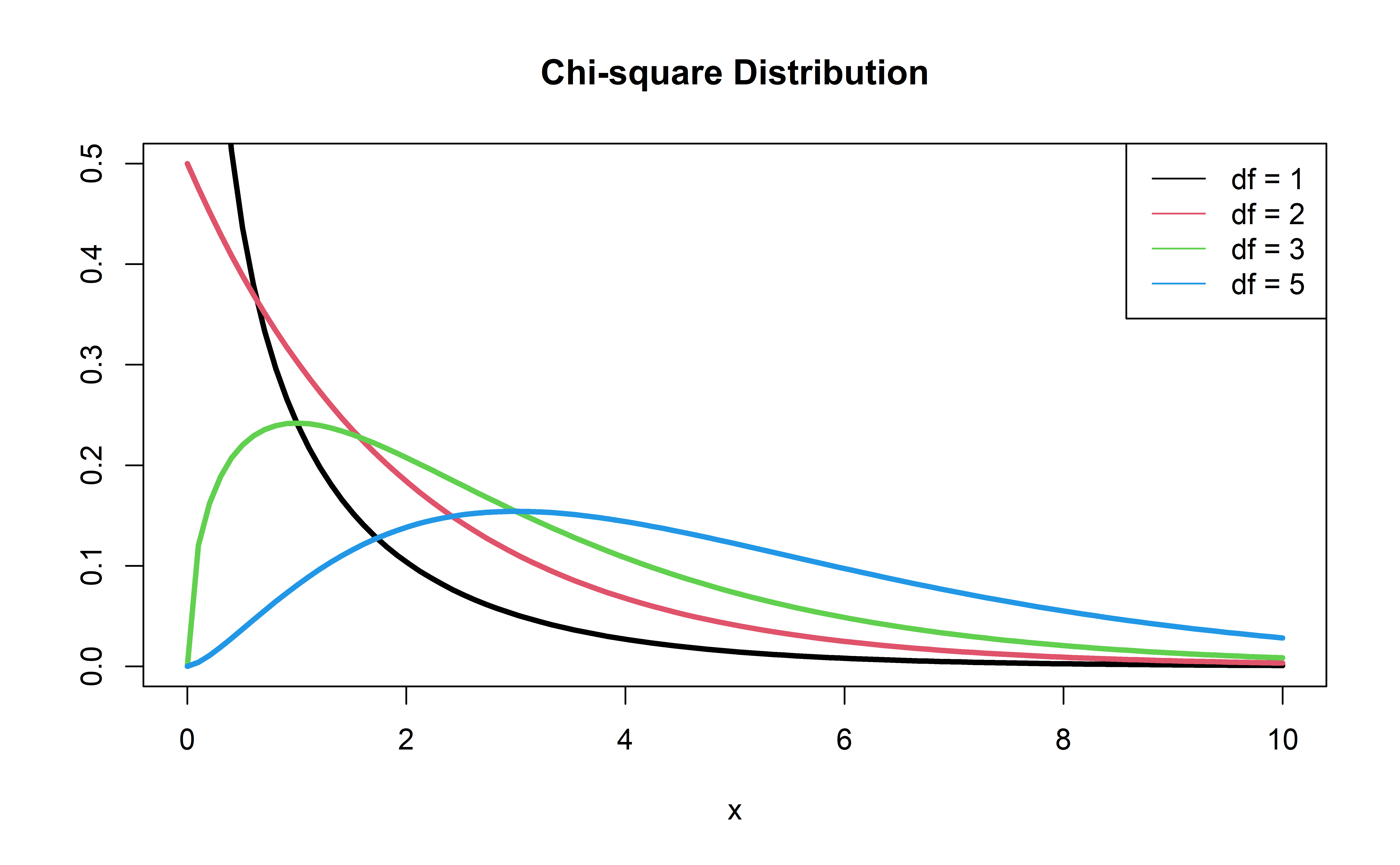
P-value: \(P(\chi^2 > G)\), calculated using a \(\chi^2\) distribution with degrees of freedom equal to the difference in the number of parameters in the full and reduced models

\(\chi^2\) distribution

Should we add `education` to a model with only `age`?

First model, reduced:

risk_fit_reduced <- glm(TenYearCHD ~ age, 
      data = heart_disease, family = "binomial")

Second model, full:

risk_fit_full <- glm(TenYearCHD ~ age + education, 
      data = heart_disease, family = "binomial")

Should we add `education` to the model?

Calculate deviance for each model:

dev_reduced <- glance(risk_fit_reduced)$deviance
dev_reduced

[1] 3306.68

dev_full <- glance(risk_fit_full)$deviance
dev_full

[1] 3300.135

Should we add `education` to the model?

Drop-in-deviance test statistic:

test_stat <- dev_reduced - dev_full
test_stat

[1] 6.544306

Should we add `education` to the model?

Calculate the p-value using a pchisq(), with degrees of freedom equal to the number of new model terms in the second model:

pchisq(test_stat, 3, lower.tail = FALSE)

[1] 0.08793145

Conclusion: The p-value is between 0.1 and 0.05 indicating mild but not strong evidence that a model with education is a useful predictor when age is already in the model.

Drop-in-Deviance test in R

We can use the anova function to conduct this test
Add test = "Chisq" to conduct the drop-in-deviance test

anova(risk_fit_reduced, risk_fit_full, test = "Chisq") |>
  tidy() |> kable(digits = 3)

term	df.residual	residual.deviance	df	deviance	p.value
TenYearCHD ~ age	4133	3306.680	NA	NA	NA
TenYearCHD ~ age + education	4130	3300.135	3	6.544	0.088

Recap

Today: Simple logistic to Multiple logistic
- Coefficient interpretations
- Wald test interpretations
- LRTs and Drop-in-Deviance tests
Basic idea add “holding all else constant”
LRT allows you to compare nested models and requires a degree of free for each extra parameter in the full model

Multiple Logistic Regression

Topics

Computational setup

Data

Risk of coronary heart disease

Data prep

Coefficient Interpretation

Model output

Model Interpretation

Model Interpretation

Inference for a single \(\beta_j\)

Hypothesis test for \(\beta_j\)

Confidence interval for \(\beta_j\)

Interpretation in terms of the odds

Coefficient for age

Coefficient for age

Coefficient for age

Coefficient for age

Comparing Nested Models

Comparing nested models

Likelihood Ratio test

\(\chi^2\) distribution

Should we add education to a model with only age?

Should we add education to the model?

Should we add education to the model?

Should we add education to the model?

Drop-in-Deviance test in R

Recap

Coefficient for `age`

Coefficient for `age`

Coefficient for `age`

Coefficient for `age`

Should we add `education` to a model with only `age`?

Should we add `education` to the model?

Should we add `education` to the model?

Should we add `education` to the model?